
Time series data shows how a metric changes over time, daily website visits, weekly sales, hourly sensor readings, or monthly customer churn. The challenge is that multiple patterns often overlap: a long-term direction, repeating seasonal cycles, and irregular shocks. STL (Seasonal-Trend decomposition using Loess) is a practical method that separates a time series into three interpretable parts: trend, seasonality, and remainder (noise). If you work with forecasting or monitoring and you’ve explored data analysis courses in Hyderabad, STL is one of the most useful tools to understand “what’s really happening” before you build models.
What STL Produces: Three Components You Can Explain
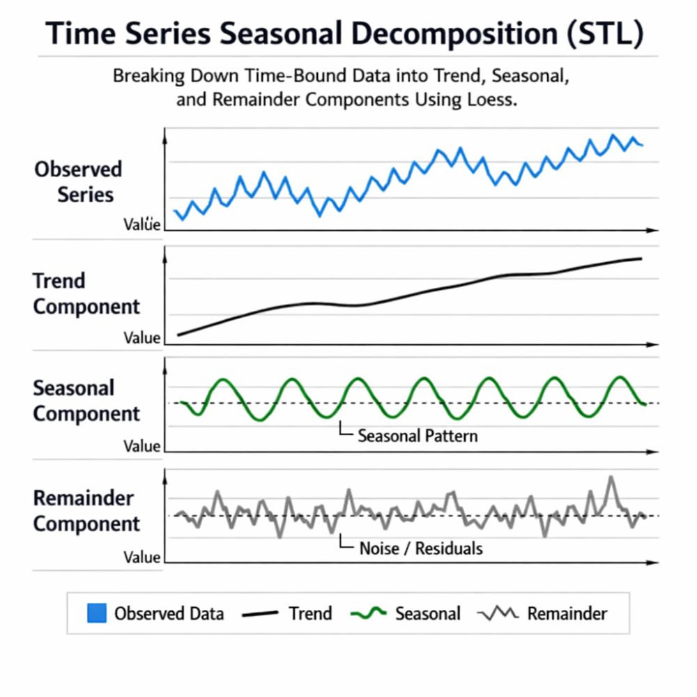
STL decomposition expresses an observed series (y) as:
- Trend (T): the smooth long-term movement (growth, decline, structural shifts)
- Seasonal (S): repeating patterns (day-of-week, month-of-year, festival effects, quarterly cycles)
- Remainder (R): what’s left after removing trend and seasonality (outliers, anomalies, random noise)
So the series becomes: y = T + S + R (additive form). This breakdown is powerful because each component can be analysed and acted upon separately. For example, a marketing team can focus on trend changes, operations can study seasonal peaks, and risk teams can inspect remainder spikes for anomalies.
How Loess Makes STL Flexible and Robust
The “engine” inside STL is LOESS (Locally Estimated Scatterplot Smoothing), a local regression method that fits simple models over small windows of time. Instead of forcing one global curve across the entire dataset, Loess adapts to local behaviour. This matters because real-world time series rarely follow neat lines; they bend, plateau, or shift due to campaigns, new product launches, policy changes, or macroeconomic effects.
STL is popular for a few reasons:
- Handles changing seasonality: seasonal patterns can strengthen, weaken, or evolve over time.
- Works well with messy data: it can be made robust to outliers, so one unusual spike doesn’t distort the decomposition.
- User control: you can tune smoothing windows to match the reality of your data rather than forcing a rigid structure.
If you’re comparing learning paths like data analysis courses in Hyderabad, STL sits at a sweet spot: it is statistically sound, but also easy to interpret for business stakeholders.
When to Use STL in Real Projects
STL is most useful when you suspect your series contains repeating cycles and you need clarity before forecasting or decision-making. Typical examples include:
- Retail or D2C sales: weekly seasonality (weekends), monthly seasonality (salary cycles), and festival-driven peaks
- Energy and utilities: daily and weekly cycles, plus weather-driven variation
- Web and app analytics: day-of-week behaviour, campaign bursts, and long-term growth trends
- Support or ticket volumes: seasonal load patterns vs sudden incident-driven surges
A practical workflow is: decompose → interpret components → handle anomalies → choose a forecasting model. Many forecasting errors happen because seasonality or outliers were not handled properly upfront.
Step-by-Step: Applying STL Correctly
Even though STL is conceptually simple, good results depend on a few disciplined steps:
1) Choose the seasonal period
You must define the season length based on your sampling frequency:
- Daily data with weekly patterns → period = 7
- Monthly data with yearly patterns → period = 12
- Hourly data with daily patterns → period = 24
If you choose the wrong period, STL will mis-allocate variance between seasonal and remainder components.
2) Check the series type (additive vs multiplicative behaviour)
If seasonal swings grow as the level grows, consider transforming the series (often a log transform). STL itself is commonly used in an additive way, and transforms help stabilise variance.
3) Enable robust fitting when outliers exist
If your series has spikes from outages, campaigns, or one-off events, robust STL reduces the influence of those points, preventing distorted trend/seasonality.
4) Validate with residual diagnostics
After decomposition, the remainder should look like “mostly noise.” If the remainder still shows patterns (e.g., repeating waves), it often means:
- the seasonal period was wrong, or
- the data has multiple seasonalities (e.g., weekly and yearly), or
- the smoothing parameters are too aggressive or too weak.
These checks are frequently emphasised in applied curricula, including data analysis courses in Hyderabad, because they directly affect forecasting accuracy and anomaly detection quality.
Interpreting the Output: What to Do with Each Component
- Trend: Use it to detect long-term growth/decline, regime changes, or the impact of strategic decisions. If the trend shifts abruptly, investigate what changed operationally or commercially.
- Seasonality: Use it for planning, staffing, inventory, infrastructure scaling, and scheduling campaigns. Seasonal peaks should not be mistaken for “true growth.”
- Remainder: Use it for anomaly detection. Large remainder values can indicate incidents, data quality problems, fraud, or unexpected external events.
A useful practice is to set alerting thresholds on the remainder rather than the raw series. This reduces false alarms caused by predictable seasonal spikes.
Conclusion
STL decomposition is a practical, stakeholder-friendly way to understand time series data by separating it into trend, seasonal, and remainder components using Loess smoothing. It improves interpretability, supports better forecasting decisions, and strengthens anomaly detection by isolating irregular behaviour from predictable cycles. If your work involves monitoring business metrics, operational load, or performance signals, and you’re exploring data analysis courses in Hyderabad, STL is a foundational technique worth mastering because it turns complex time-bound data into clear, actionable insight.
Related Posts